Adding XPBD-Based Rigid Body Physics to ToyMaker

I decided to add physics to my game engine, now named “ToyMaker,” based on Extended Position Based Dynamics.

What is a physics engine?

So a game – specifically a modern realtime 3D computer game – is, at its heart, a piece of software like any other. It holds a big bag of data relating to the purpose of the game, and it allows a user to modify that data in strictly controlled ways, periodically showing them the results of their modifications.

The physics engine is the system in the game that attempts to model physical phenomena, i.e., forces causing a change in an object’s velocity, and the object’s velocity causing a change in its position, etc. In order to represent a particular “physical” object, then, we might have:

• The object’s position (as a list of 3 floats) and orientation (as a 4 float quaternion).

• The kinematic properties of the object, i.e., its positional and angular velocities, each as a list of 3 floats.

• The forces acting on the object, represented as the sum force acting on its center of mass, and the sum torque around an axis passing through its center of mass, also as 3 float vectors.

• The physical properties of the object – its mass, rotational inertia, static and dynamic friction coefficients, its shape, and so on.

We might choose to represent this data in a kind of table, like so:

Name	Type	Value
pos	flt3	0, 0, 5
ori	quat	1, 0, 0, 0
vel	flt3	0, -1, 0
aVel	flt3	0, 0, 0
frce	flt3	0, -10, 0
trq	flt3	0, 0, 0
mass	flt	1
sFrc	flt	0.3
dFrc	flt	0.2
shp	enum	SPHERE
rdus	flt	1.0

… which is indeed somewhat close to how our computer program “sees” this object.

A part of what separates computer games from other kinds of software is that the state of the game – all represented in tables much like the one above – is advanced several times each second, with or without input from the user. Those states are displayed to the user tens of times each second too, in the form of rapidly changing images, to give the appearance of movement.

The physics engine performs these updates for the physical state of the simulation by dividing time into a series of discrete time steps; for a physics engine running at 60Hz, this would be a timestep of ~16 milliseconds, or 0.016 seconds. At each step, the engine asks “Given that this object is here right now, where should it be in the next 1/60th of a second?”, which it then answers using formulae derived from Newtonian mechanics.

Here’s what that looks like for some of the values from the table above, in a single time step.

Name	Type	Value
vel	flt3	0, -1.16, 0
pos	flt3	0, 0, 4.98144

Where:

• the velocity update:
  1. newVel = vel + frce * timestep / mass
  2. newVel = (0, -1, 0) + (0, -10, 0) * 0.016 / 1.0
  3. newVel = (0, -1.16, 0)
• the position update:
  1. newPos = pos + newVel * timestep
  2. newPos = (0, 5.0, 0) + (0, -1.16, 0) * 0.016
  3. newPos = (0, 4.98144, 0)

Picture such an update happening 60 times a second for this object and every other “physical” object in the game, and you now have a rough idea of what a physics engine does.

The physics update

Physics state

We’ve already seen the table representing most of the data that we’ll want to associate with an object. ToyMaker’s ObjectBounds component, already provides a representation for the shape, position, and orientation of the object, so our first task is to make a struct for the object’s other physical properties.

Here’s what that struct looks like, with some omissions for simplicity:

struct PhysicsState {
    /**
     * @brief The sum of all the forces acting on this object's center of mass,
     * causing it to move through space.
     *
     * Expressed as a vector in the world frame.
     *
     */
    glm::vec3 mForce { 0.f };

    /**
     * @brief Proportional to sum of all forces acting perpendicular to the vector going
     * from the point at which the forces are being applied to this object' center of
     * mass, causing it to rotate about its axis.
     *
     * Expressed as a vector in the world frame.
     *
     */
    glm::vec3 mTorque { 0.f };

    /**
     * @brief The velocity of this object.
     *
     * Expressed as a vector in the world frame.
     *
     */
    glm::vec3 mVelocity { 0.f };

    /**
     * @brief The angular velocity of this object.
     *
     * Expressed as a vector in the world frame.
     *
     */
    glm::vec3 mAngularVelocity { 0.f };

    /**
     * @brief The inverse of this object's resistance to rotational change.
     *
     * Expressed in terms of the object's local frame, and should be derived from
     * the object's mass and shape.
     *
     */
    glm::vec3 mRotationalInertiaInverse { 1.f };

    /**
     * @brief The inverse of this object's mass.
     *
     */
    float mMassInverse { 1.f };

    /**
     * @brief The friction coefficient of the force that prevents relative motion between the
     * surface of two objects when they are stationary.
     *
     */
    float mCoefficientFrictionStatic { 0.f };

    /**
     * @brief The friction coefficient of the force that hinders motion between the surface of
     * two objects when they are moving relative to each other.
     *
     */
    float mCoefficientFrictionDynamic { 0.f };
};

You can find a more complete description of the struct here.

The integration function

Now that we have a representation for our object’s physics state, our next task is to write an integration function – also called a “prediction step” in XPBD – to get our objects moving. The integration function is called once per timestep, and looks something like this:

1. For each object:

   1. Using the sum of forces acting on the center of mass of the object, compute the change to its velocity, and add it to the object’s previous velocity to find its new velocity.

   2. Using the sum of torques acting on the object, compute the change to its angular velocity, and add the change to its previous angular velocity to find its new angular velocity.

   3. Using the velocity of the object, compute and apply the change to the object’s position in this timestep.

   4. Using the angular velocity of the object, compute and apply the change to the object’s orientation in this timestep.

Note

Integration means something like “accumulation,” for those not terribly comfortable with calculus terms. In our example from the previous section we used a formula to discover, given a force acting on an object’s center of mass, the change to that object’s velocity for a fixed quantity of time, which we then added to the object’s previous velocity in order to obtain its new velocity.

We did a similar thing with the object’s velocity as well, where we added the change in position due to its velocity for a fixed quantity in time to the object’s old position to obtain its new position.

The addition of a quantity representing some change, to another quantity representing an accumulation of such changes, is what we might call “integration.”

In ToyMaker::PhysicsSystem::integrateForces(), that looks something like this:

for(auto entity: mEntities) {
    auto physics { getComponent<PhysicsState>(entity) };
    auto bounds { getComponent<ObjectBounds>(entity) };

    // update positional and rotational velocities based on external forces
    physics.mVelocity += timestepSeconds * physics.mForce * physics.mMassInverse;
    const glm::quat orientation { bounds.getOrientationWorld() };
    const glm::quat toLocal { glm::inverse(bounds.getOrientationWorld()) };
    const glm::vec3 rotationalInertiaLocal { physics.getRotationalInertia() };
    const glm::vec3 angularVelocityLocal { toLocal * physics.mAngularVelocity };
    const glm::vec3 torqueLocal { toLocal * physics.mTorque };
    const glm::vec3 deltaAngularVLocal { timestepSeconds
        * physics.mRotationalInertiaInverse * (
            torqueLocal - glm::cross(
                angularVelocityLocal,
                rotationalInertiaLocal * angularVelocityLocal
            )
    ) };
    physics.mAngularVelocity += orientation * deltaAngularVLocal;

    // update position and orientation based on velocities
    const float deltaAngle {
        timestepSeconds * glm::length(physics.mAngularVelocity)
    };
    const glm::vec3 axisAngularVelocity { glm::normalize(physics.mAngularVelocity) };
    const glm::quat orientationUpdate { glm::angleAxis(deltaAngle, axisAngularVelocity) };
    const auto newOrientation { glm::normalize(orientationUpdate * physicsState.mBounds.getOrientationWorld()) };
    bounds.setOrientationWorld(newOrientation);
    bounds.setPositionWorld(
        physicsState.mBounds.getPositionWorld() + timestepSeconds * physics.mVelocity
    );

    updateComponent(entity, physics);
    updateComponent(entity, bounds);
}

This is what we get as a result:

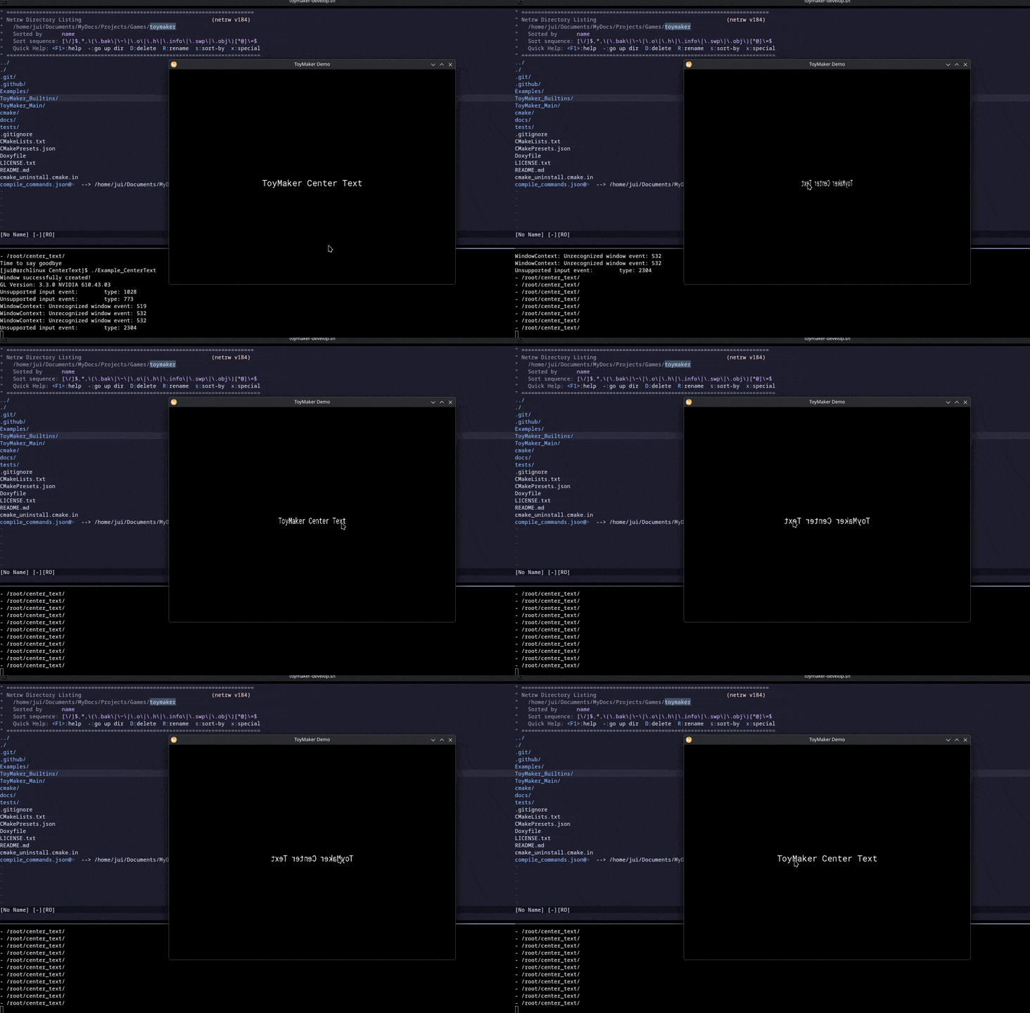
Here we see pointer clicks applying a force to a text object fixed at its center, causing it to spin. The applied forces cause a change to the object’s angular velocity, which in turn causes the object’s orientation to change. In this example, the physics update runs at a rate of 30Hz, or 30 times each second.

Here’s a clip of two balls colliding:

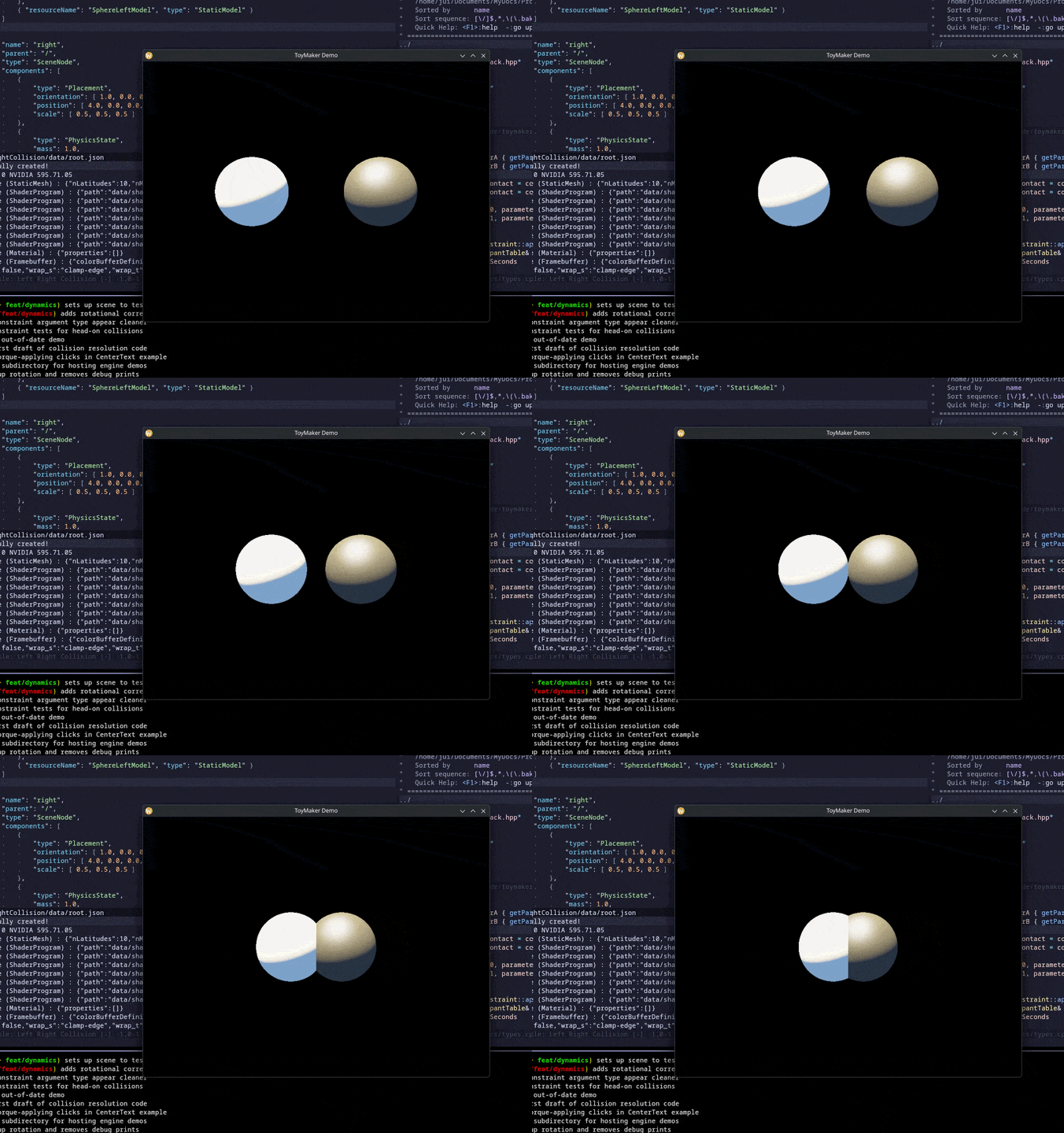
… well, not really. There are a couple of problems here:

1. Visually, it’s quite clear to us that the two balls are intersecting, and that they shouldn’t. But try to imagine what the computer sees. Or better still, take a look:

   Name	Type	Value
   pos1	flt3	-0.836, 0, 0
   pos2	flt3	0.836, 0, 0
   ori1	quat	1, 0, 0, 0
   ori2	quat	1, 0, 0, 0
   shp1	enum	SPHERE
   shp2	enum	SPHERE
   rdus1	flt	1.0
   rdus2	flt	1.0

   The fact that the balls in the demo are intersecting is slightly more difficult to see in this form. Even if we are able to apply our knowledge of geometry to answer questions about whether these spheres in particular are intersecting, how would we handle other shapes?

   Turns out that there’s a very popular pair of algorithms that helps us answer intersection questions for all convex shapes: GJK, to determine whether a pair of convex shapes is intersecting, and EPA, to find, for each object in the pair, its point of contact, and the distance and direction the object would need to move in order to be separated from the other object.

   Note

   Concave shapes are usually represented as groups of convex shapes in realtime physics engines. That means that this pair of algorithms can help us represent and use any sensible 3D shape we can imagine in our physics engine.

   Check the links at the end of this post.

2. Assuming that we can get our hands on information about the contact, how do we modify the motion of the objects such that they believably comply with physical laws?

XPBD

What are constraint solvers?

Computer simulations that attempt to model physical phenomena use a class of algorithms called constraint solvers. The basic idea here is that, while it is difficult to entirely prevent inaccuracies (or errors) in realtime simulations, what we can more easily do is:

1. Discover the error when it occurs:

   • In our earlier example, an intersection between two shapes occurred (which we know shouldn’t happen, making it an error), and we were able to determine the location, direction, and magnitude of the intersection.

   • We might model the extension of a spring as an error relative to its rest length.

   • We could also class the change in volume of a deformable object as an error relative to its original volume.

   • Angular errors can be computed this way too. An overbent joint (picture a broken elbow) is an error relative to the angular limits of that joint.

2. Then, either:

   1. Compute the forces it would take to effect a correction to the objects involved in the error in as few steps as possible, then apply them to the objects, resolving the error during our usual physics integration step.

   2. Apply position corrections to the objects right away, and derive what forces would have caused the correction after the correction has been applied (if required).

The former approach is the one that has been popular in the kind of realtime physics simulations we’ve seen in video games for a long time. This type of constraint solver is called an impulse-based solver. While there’s plenty of material talking about this approach, I haven’t studied it and so can’t really comment. From what I understand, Brian Mirtich’s Impulse-based Dynamic Simulation of Rigid Body Systems – 1996 is the place to start learning about them.

Detailed Rigid Body Simulation with Extended Position Based Dynamics - Matthias Müller, Miles Macklin, Nuttapong Chentanez, Stefan Jeschke, Tae-Yong Kim takes the latter approach, immediately applying corrections to bodies in error relative to some constraint, and deriving correction forces post-hoc per need. This paper was the primary basis of my implementation, along with several videos from Matthias’ Ten Minute Physics collection of videos.

Collision constraints

Collision response data

Let’s go back to our example scene. We have two shapes – in this case, spheres – colliding. The spheres begin to intersect one another while moving towards each other. We have a way to detect and quantify their overlap in GJK and EPA.

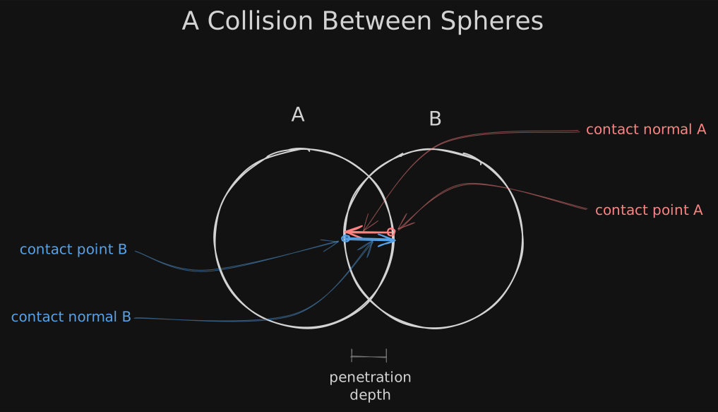
The data generated here is called the collision response data corresponding to a pair of overlapping objects. In English, this is what the labels mean:

• contact point: For each object, a point on its surface that penetrates the furthest into the other colliding shape.

• contact normal: For each object, the direction in which it would have to move in order to no longer overlap with the other object.

• penetration depth: For either object, the shortest distance the object would need to move along its contact normal to no longer overlap with the other.

As C++ structs taken from ToyMaker::Contact:

/**
 * @brief Object representing contact information between a pair of convex shapes from the
 * perspective of _one_ of those shapes.
 *
 * All 3D points and vectors are given relative to the world.  Additional processing of
 * this data is necessary to convert them to local-space data.
 *
 */
struct Contact {
    /**
     * @brief The worldspace point on the surface of this shape that made contact with the other shape
     *
     */
    glm::vec3 mPoint;

    /**
     * @brief Worldspace normal pointing inward from the surface of this
     * shape such that moving in this direction by the penetration depth
     * will remove the overlap.
     */
    glm::vec3 mNormal;

    /**
     * @brief The length by which to move this object in the direction of
     * the contact normal to separate the colliding objects
     *
     */
    float mPenetrationDepth;
};

/**
 * @brief Data representing everything about a collision.
 *
 * This data includes:
 *
 * - Contact information relative to each object, referred to as A and
 * B, depending on the order of parameters passed to the collision evaluator
 *
 */
struct Collision {

    /**
     * @brief Contact information relative to the _first_ collision shape
     *
     */
    Contact mContactA;

    /**
     * @brief Contact information relative to the _second_ collision shape
     *
     */
    Contact mContactB;
};

Computing Gauss-Seidel update terms

Per the paper, our collision constraint is a positional constraint, meaning that the points participating in the constraint – here, the contact points – must be moved through space to comply with the constraint again. In XPBD, this occurs through a step called a projected Gauss-Seidel update.

For a general position constraint involving 2 participants, we compute a scalar value the paper calls a Lagrange multiplier update, whose formulae are rendered in C++ syntax below:

// before the first position solve:
float lambda = 0.f;

// ...

// for every other solve, for all active constraints
const float deltaLambda = (
    (
        -c - alpha / (timestep * timestep) * lambda
    ) / (
        w_1 + w_2 + alpha / (timestep * timestep)
    )
);
lambda += deltaLambda

The general method to determine the equation for the update for any positional physical constraint, given a way to measure error, is described briefly in Matthias’ video of the XPBD technique. In the context of our collision correction:

• We can conveniently ignore compliance related terms, labelled alpha in the paper, since our collision related constraints will always have a compliance of 0.

• We treat the penetration depth of the collision as the error in the collision constraint. In the paper, this is the c term in equation (4).

• For each object, the negative of the contact normal gives us the direction of the greatest increase in error, which I’ll call the correction direction. The paper labels this term n in equations (2), (3), (10), etc.

• We can compute the generalized inverse mass for each object as below. In the paper these are terms w_1 and w_2 in equations (2) and (3).

   float computeGeneralizedInverseMassPositional(
       const ObjectBounds& object,
       const PhysicsState& physics,
       const glm::vec3& correctionPoint,
       const glm::vec3& correctionGradient
   ) {
       const glm::vec3 position { object.getPositionWorld() };
       const glm::vec3 correctionOffset { correctionPoint - position };
       const glm::vec3 correctionRotational { glm::cross(correctionOffset, correctionGradient) };
       const float generalizedInverseMass { physics.mMassInverse + (squareDistance(correctionRotational)?
           computeGeneralizedInverseMassRotational(
               object, physics, correctionRotational
           ) : 0.f)
       };
       return generalizedInverseMass;
   }
  
   float computeGeneralizedInverseMassRotational(
       const ObjectBounds& object,
       const PhysicsState& physics,
       const glm::vec3& correction
   ) {
       const glm::quat orientation { object.getOrientationWorld() };
       const glm::vec3 correctionLocal { glm::inverse(orientation) * correction };
       return glm::dot(correctionLocal, physics.mRotationalInertiaInverse * correctionLocal);
   }
  

  Here, correctionPoint refers to the point on the surface of the object participating in the constraint. In our collision constraint, this would be the object’s contact point with the other object.

  correctionGradient is a vector along n representing the offset from the constrained point’s current position that it would need to move in order to increase error c by exactly one unit.

  For our collision constraint, this is a vector of magnitude one, and therefore the same as direction vector n.

• The Lagrange multiplier delta – deltaLambda in equations (4) and (5) of the paper, and implicitly in eqns., (6) onwards – is a quantity representing the impulse that must be applied to the colliding objects to perform the correction.

   const float lagrangeDeltaCollision {
       -mPenetrationDepth / (
           generalizedInverseA + generalizedInverseB
       )
   };
  

  Note:

  Here, my implementation diverges from the paper.

  In equations (10) and onwards, the paper uses lambda. For collision constraints, I find thatlambda gives overly large values for contact forces, while deltaLambda produces more reasonable ones. This is particularly important when it comes to computing frictional forces and restitution corrections.

  I’m not sure whether lambda is the quantity used, or whether every instance of lambda should be interpreted as deltaLambda in general.

• We take the Lagrange multiplier delta scalar and correction direction vector together to get the positional correction impulse.

   const glm::vec3 positionalImpulse { lagrangeDeltaCollision * mContactNormal };
  

Applying the positional correction

The positional impulse is applied as-is to the center of mass of the object. The rotational component of the correction is computed by its cross product with the relative offset of the contact point from the object’s center of mass. Overall, the update looks something like this:

ObjectBounds applyImpulseObject(
    ObjectBounds object,
    const PhysicsState& physics,
    const glm::vec3& impulsePositional,
    const glm::vec3& impulsePoint
) {
    // apply positional corrections
    const glm::vec3 position { object.getPositionWorld() };
    const glm::vec3 positionNew { position + impulsePositional * physics.mMassInverse };
    object.setPositionWorld(positionNew);

    // apply rotational corrections
    const glm::vec3 impulseRotation { glm::cross(
        impulsePoint - position, impulsePositional
    ) };
    object = applyImpulseObject(object, physics, impulseRotation);
    return object;
}

ObjectBounds applyImpulseObject(
    ObjectBounds object,
    const PhysicsState& physics,
    const glm::vec3& impulseRotational
) {
    const glm::quat orientation { object.getOrientationWorld() };
    const glm::vec3 impulseRotationalLocal { glm::inverse(orientation) * impulseRotational };
    const glm::vec3 deltaOrientation { orientation * (physics.mRotationalInertiaInverse * impulseRotationalLocal) };
    const glm::quat orientationNew { glm::normalize(
        orientation + .5f * glm::quat(0.f, deltaOrientation.x, deltaOrientation.y, deltaOrientation.z) * orientation
    ) };
    object.setOrientationWorld(orientationNew);
    return object;
}

Note

While not covered here, separating the rotational part of the position correction out from the positional part allows us to reuse the rotational correction function for generic angular constraints.

Modifications to the physics update

Now that we know how to compute values for terms participating in the Gauss-Seidel update, we can talk about the changes we need to make in our physics update.

The first change relates to our timestep. Traditionally, constraint solvers would iterate through all active constraints several times until the total error across constraints had been minimized (or until the solver ran out of iterations). The paper advises against this. Instead, it recommends subdividing the physics timestep into smaller substeps. According to the paper, this improves the accuracy of the simulation and its time to convergence.

The other change will of course be the addition of the position constraint solve itself.

Accordingly, we get:

1. For each substep, where substep = timestep / numSubsteps:

   1. For each object:

      1. Integrate forces.

      2. Apply collision (position) constraints.

      3. Derive actual object velocities after the position correction.

Where the collision constraint algorithm is:

1. Get the collision response data for a pair of intersecting objects.

2. Compute the generalized inverse mass for each object.

3. Use collision data to compute a Lagrange multiplier delta.

4. Use the Lagrange multiplier delta to compute a positional correction impulse.

5. Apply the correction impulse (in opposing directions) to both objects.

Overall, this gives us an update that looks like this:

// high level physics update
void PhysicsSystem::onSimulationStep(uint32_t timestepMillis) {
    // subdivide our physics timestep (and convert to seconds)
    const float substepInterval { (static_cast<float>(timestepMillis) / static_cast<float>(mSubsteps)) / static_cast<float>(1e3) };

    // collect all potential collisions
    collectPotentialCollisions(substepInterval);

    // refresh lagrange multipliers for ongoing collisions
    for(auto& constraint: mCollisionConstraints) {
        collisionConstraint.second.resetLagrange();
    }

    for(auto substep { 0 }; substep < mSubsteps; ++substep) {
        integrateForces(substepInterval);

        // this updates the collision response data stored along with
        // each collision constraint using GJK and EPA
        detectCollisions();

        applyPositionConstraints(substepInterval);

        // we'll talk about this soon!
        deriveVelocities(substepInterval);
    }
}

void PhysicsSystem::applyPositionConstraints(float substepInterval) {
    // apply non-collision constraints (not shown here)

    // ...

    // solve collision constraints
    for(auto& collisionPairConstraint: mCollisionConstraints) {
        const auto& collisionEntities { collisionPairConstraint.first };
        auto& collisionConstraint { collisionPairConstraint.second };

        const auto entityA { collisionPairConstraint.first.first };
        const auto entityB { collisionPairConstraint.first.second };

        auto objectA { getComponent<ObjectBounds>(entityA) };
        auto objectB { getComponent<ObjectBounds>(entityB) };
        auto physicsA { getComponent<PhysicsState>(entityA) };
        auto physicsB { getComponent<PhysicsState>(entityB) };

        collisionConstraint.applyConstraintPosition(objectA, physicsA, objectB, physicsB);
    }
}

// application of a single positional constraint
void CollisionConstraint::applyConstraintPosition(
    ObjectBounds& objectA, PhysicsState& physicsA,
    ObjectBounds& objectB, PhysicsState& physicsB
) {
    const glm::vec3 positionA { objectA.getPositionWorld() };
    const glm::vec3 positionB { objectB.getPositionWorld() };
    const glm::quat orientationA { objectA.getOrientationWorld() };
    const glm::quat orientationB { objectB.getOrientationWorld() };

    // compute generalized inverse masses for A and B -- these will
    // be recomputed each substep, so there's no point in storing them
    const float generalizedInverseA { computeGeneralizedInverseMassPositional(
        objectA,
        physicsA,
        mLastPointContactA,
        mContactNormal
    ) };
    const float generalizedInverseB { computeGeneralizedInverseMassPositional(
        objectB,
        physicsB,
        mLastPointContactB,
        mContactNormal
    ) };

    // compute correction value
    const float lagrangeCollision { getLagrange().at(0) };
    const float lagrangeDeltaCollision {
        -(
            mPenetrationDepth
        ) / (
            generalizedInverseA + generalizedInverseB
        )
    };
    applyLagrangeDelta(lagrangeDeltaCollision, 0);
    const glm::vec3 positionalImpulse {
        lagrangeDeltaCollision * mContactNormal
    };

    // apply corrections
    objectA = applyImpulseObject(
        objectA,
        physicsA,
        positionalImpulse,
        mLastPointContactA
    );
    objectB = applyImpulseObject(
        objectB,
        physicsB,
        -positionalImpulse,
        mLastPointContactB
    );

    updateComponent(entityA, objectA);
    updateComponent(entityB, objectB);
}

Note

The actual implementation contains a lot of tech debt and architectural cruft which I’ve omitted here.

We also need to derive velocities after the position correction.

// high level physics update
void PhysicsSystem::onSimulationStep(uint32_t timestepMillis) {
    for(auto substep { 0 }; substep < mSubsteps; ++substep) {
        // everything else

        // ...

        // !!!!!!!! this thing:
        deriveVelocities(substepInterval);
    }
}

The problem here is that we might have a hundred positional constraints affecting the same object. Imagine one ball among several balls gradually filling a basket, for example.

Our position constraint prevents the ball from intersecting with the other balls and from escaping the basket, but it does not modify the motion of the ball, meaning that the ball will continue to try to move in the same direction as before the collision. In the code snippets shown thus far, we don’t touch PhysicsState::mVelocity or PhysicsState::mAngularVelocity.

deriveVelocities() is responsible for this instead. It measures the changes in positions and orientations of each object in the simulation, and along with the substep interval uses these measurements to tell what the object’s velocities actually are. These are 3D versions of velocity = (position2 - position1) / time and angularVelocity = (angle2 - angle1) / time.

First, we need to cache object properties prior to the position solve.

void PhysicsSystem::integrateForces(float substepSeconds) {https://www.britannica.com/science/kinetic-friction
    // all the other stuff

    // ...

    mPreviousStates[entity].mPhysics = physics;
    mPreviousStates[entity].mBounds = bounds;
}

Then, we can solve for the object’s new velocities:

void PhysicsSystem::deriveVelocities(float substepSeconds) {
    for(const auto entity: getEnabledEntities()) {

        // retrieve current and previous states
        auto physics { getComponent<PhysicsState>(entity) };
        const auto bounds { getComponent<ObjectBounds>(entity) };
        const auto orientationInverse { glm::inverse(bounds.getOrientationWorld()) };
        const auto& previousState { mPreviousStates[entity] };

        // update linear terms
        physics.mVelocity = (
            (bounds.getPositionWorld() - previousState.mBounds.getPositionWorld())
            / substepSeconds
        );

        // update angular terms
        const glm::quat deltaOrientation {
            (bounds.getOrientationWorld() * glm::inverse(mPreviousStates.mBounds.getOrientationWorld()))
        };
        physicsProps.mAngularVelocity = (2.f * glm::vec3 {
            deltaOrientation.x, deltaOrientation.y, deltaOrientation.z
        } / substepSeconds);
        physicsProps.mAngularVelocity *= deltaOrientation.w >= 0.f ? 1.f : -1.f;

        updateComponent(entity, physics);
    }
}

Note

We didn’t need this before because an object’s external forces, its velocity, and its position and orientation, all had a simple one-to-one relationship with each other when we only had the prediction step.

The position and orientation changes introduced by the position constraint break that relationship.

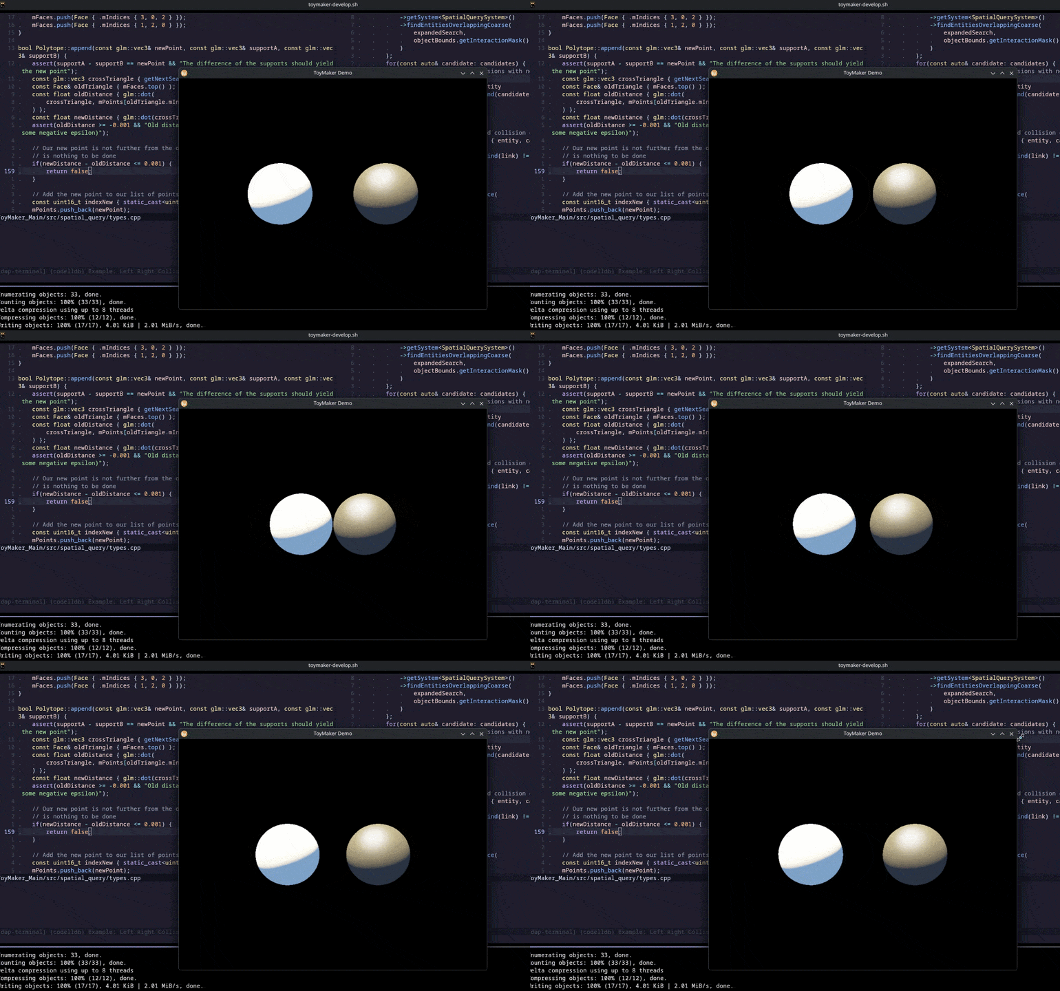
This finally allows our spheres to actually collide, then bounce away from each other!

Friction constraints

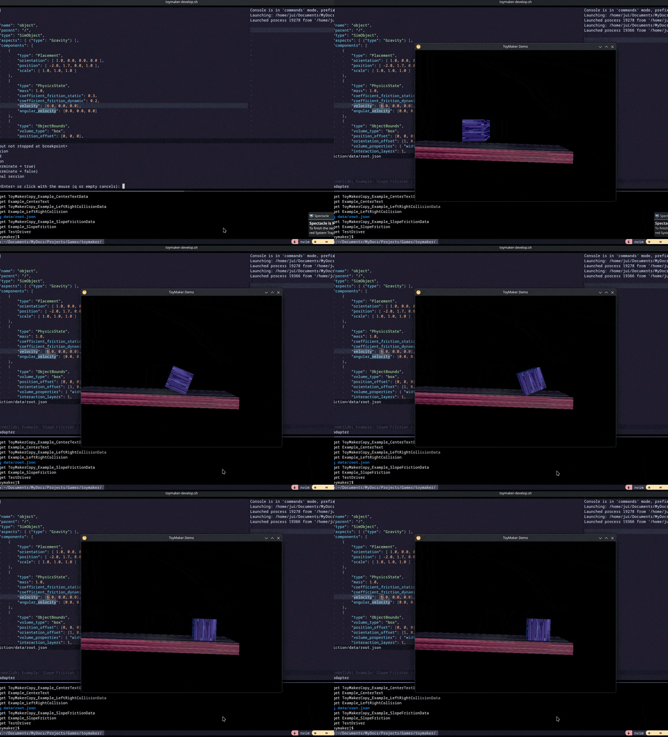
We aren’t done yet. Take a look at this clip.

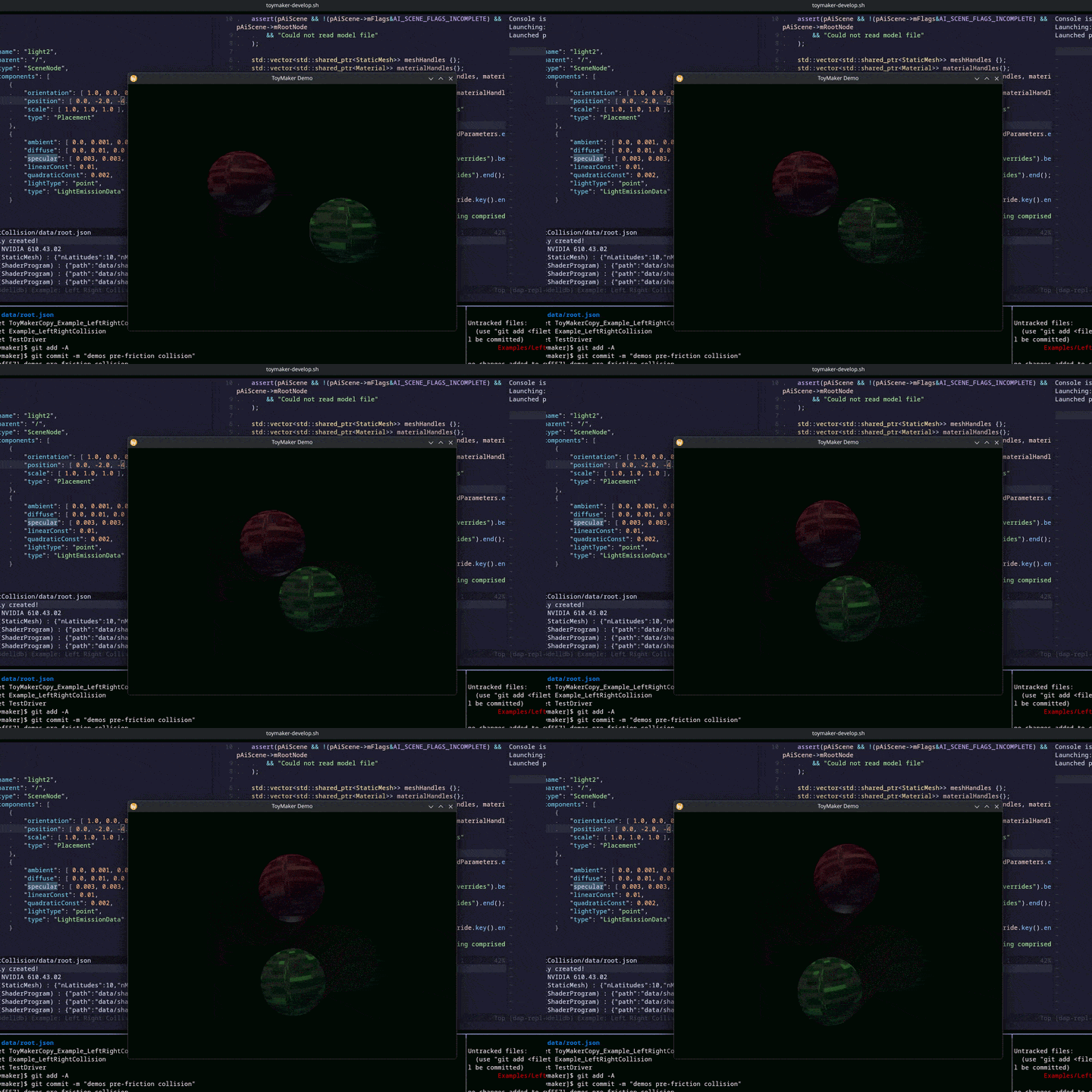
And this one.

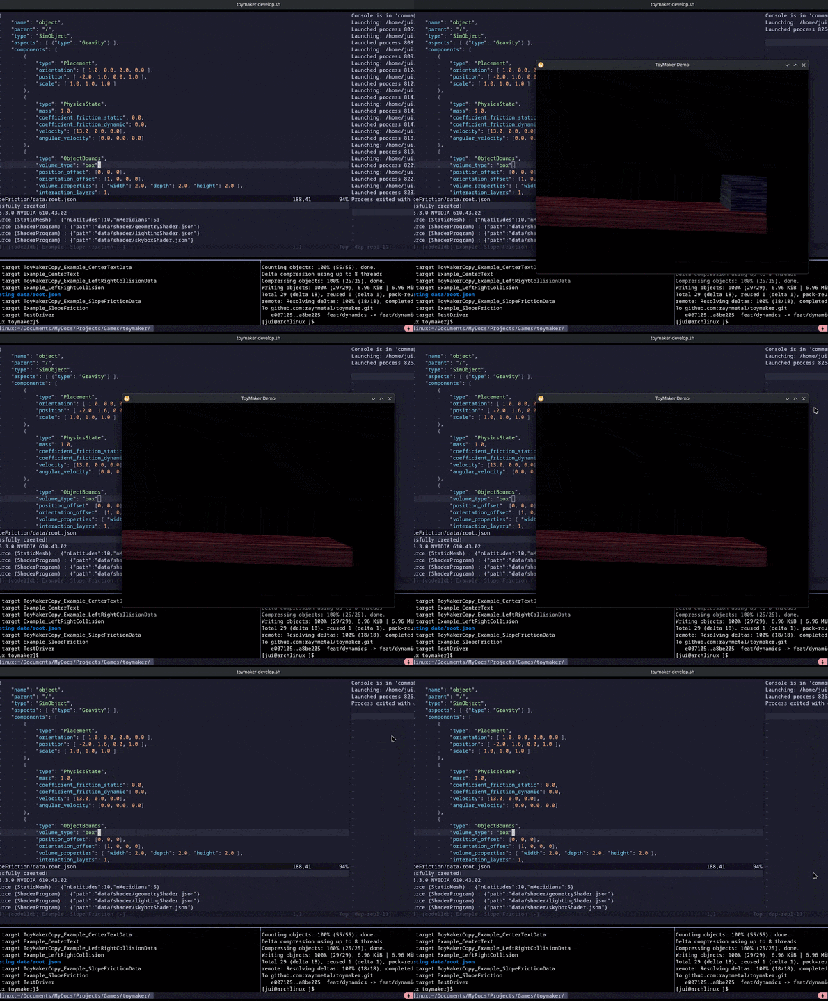
Note:

The incline is tagged by the physics system as a static object. This causes the physics system to exclude it from velocity and position updates, while still allowing dynamic objects to collide with it. It is treated as an object with infinite mass during these collisions.

Most physics engines do this kind of tagging for the objects in the scenes they manage, reserving expensive physics updates strictly for those objects that require it.

If all the world was made of ice or bowling ball alleys, there would be nothing particularly wrong with this. I want more than that, though, so we’ll need to add friction constraints.

There are two kinds of friction forces:

• Static friction attempts to prevent relative tangential motion between two bodies at their point of contact.

• Dynamic friction opposes relative tangential motion that is already taking place between two objects, again at their point of contact.

In XPBD, the first is modeled as a position constraint, very like the one we used for the collision itself. The second is modeled through something called a velocity constraint. Sections 3.5 and 3.6 of the paper talk about this.

Static friction

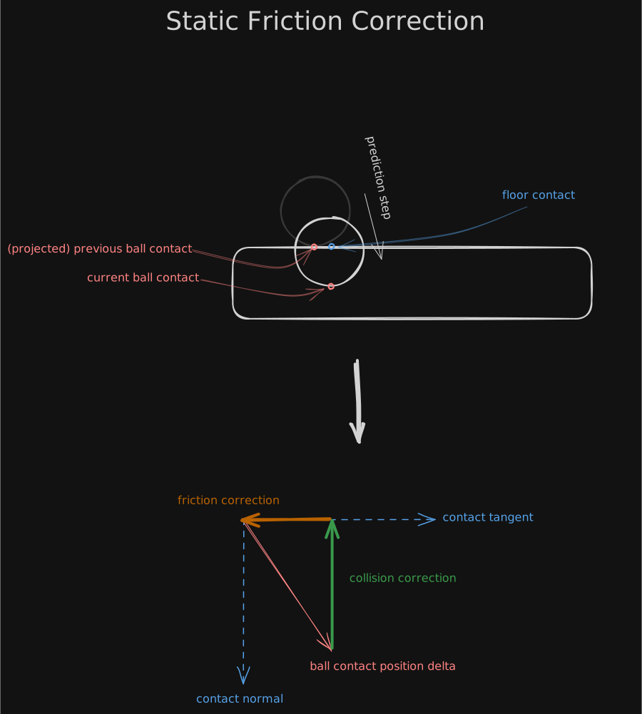
When a force attempts to move an object tangentially, relative to another object, a static friction force exactly equal to that force in the opposite direction arises and prevents this motion, up to some threshold given by mu_static * normalForce, where mu_static is the static friction coefficient between the surfaces of the two objects.

After the collision correction, we can find the vector representing the tangential change in the position of the contact point.

// called before the physics update, as part of detectCollisions()
void CollisionConstraint::updateCollisionData(
    const Collision& collision,
    const PhysicsState& physicsA, const ObjectBounds& boundsA, const ObjectBounds& boundsAPrev,
    const PhysicsState& physicsB, const ObjectBounds& boundsB, const ObjectBounds& boundsBPrev
) {
    mCurrentPointContactA = collision.mContactA.mPoint;
    mCurrentPointContactB = collision.mContactB.mPoint;
    mRelativePointContactA = (
        glm::inverse(boundsA.getOrientationWorld()) * (
            collision.mContactA.mPoint - boundsA.getPositionWorld()
        )
    );
    mRelativePointContactB = (
        glm::inverse(boundsB.getOrientationWorld()) * (
            collision.mContactB.mPoint - boundsB.getPositionWorld()
        )
    );

    // we project the contact point to its position in the last frame so that
    // we have a point of comparison for it
    mLastPointContactA = (
        boundsAPrev.getPositionWorld()
        + boundsAPrev.getOrientationWorld() * mRelativePointContactA
    );
    mLastPointContactB = (
        boundsBPrev.getPositionWorld()
        + boundsBPrev.getOrientationWorld() * mRelativePointContactB
    );

    // ...

    // other stuff
}

void CollisionConstraint::applyConstraintPosition(/* args */) {
    // collision position constraint applied

    // ...

    // derive relative motion of point of contact
    const glm::vec3 pointContactANew { positionANew + orientationANew * mRelativePointContactA };
    const glm::vec3 pointContactBNew { positionBNew + orientationBNew * mRelativePointContactB };
    const glm::vec3 deltaA { pointContactANew - mLastPointContactA };
    const glm::vec3 deltaB { pointContactBNew - mLastPointContactB };
    const glm::vec3 deltaAB { deltaA - deltaB };
    const glm::vec3 deltaABTangent {
        deltaAB - glm::dot(deltaAB, mContactNormal) * mContactNormal
    };

    // ...

    // other stuff
}

When static friction is in effect, deltaABTangent should be 0. Accordingly, we can directly use deltaABTangent’s direction and magnitude as the direction and magnitude of the position correction.

void CollisionConstraint::applyConstraintPosition(/* args */) {
    // other stuff

    // ...

    const float lagrangeDeltaFriction {
        -(
            glm::length(deltaABTangent)
        ) / (
            generalizedInverseA + generalizedInverseB
        )
    };
    const glm::vec3 positionalImpulseFriction {
        lagrangeDeltaFriction * glm::normalize(deltaABTangent)
    };

    // ...

    // more stuff
}

In our collision correction, we have a quantity lagrangeDeltaCollision proportional to the force along the contact normal between the two surfaces. Conveniently, this means that any inequality that applies to the forces themselves also applies to this quantity. Accordingly, we apply a positional correction only when mu_static * lagrangeDeltaCollision >= lagrangeDeltaFriction:

void CollisionConstraint::applyConstraintPosition(/* args */) {
    // other stuff

    // ...

    if(
        !lagrangeDeltaFriction || (
            glm::abs(lagrangeDeltaFriction)
            >= glm::abs(combinedFrictionCoefficient * lagrangeDeltaCollision)
        )
    ) {
        return;
    }

    // apply corrections
    objectA = applyImpulseObject(
        objectA,
        physicsA,
        positionalImpulseFriction,
        pointContactANew
    );
    objectB = applyImpulseObject(
        objectB,
        physicsB,
        -positionalImpulseFriction,
        pointContactBNew
    );

    updateComponent(entityA, objectA);
    updateComponent(entityB, objectB);
}

Note:

For the combinedFrictionCoefficient, we can choose to use the average of the coefficient of friction of both objects, or their minimum, or their maximum. In my implementation, I use the minimum.

Dynamic friction

Dynamic friction (also, kinetic friction) opposes the relative motion of two objects in contact with each other. In XPBD, this force is modeled as a velocity constraint. This means that rather than changing the object position, then seeing the result of the correction in the velocity derivation step, we directly modify the velocity to perform the constraint correction.

Once we’ve derived the velocities for the two participants, we measure the distance moved by their relative points of contact to find their relative tangential velocity.

void CollisionConstraint::applyConstraintVelocity(/* args */) {
    // other stuff

    // ...

    // discover just how fast the contact points on each surface are moving
    // relative to each other
    const glm::vec3 pointVelocityA { physicsA.mVelocity + glm::cross(
        physicsA.mAngularVelocity,
        contactPositionA - positionA
    ) };
    const glm::vec3 pointVelocityB { physicsB.mVelocity + glm::cross(
        physicsB.mAngularVelocity,
        contactPositionB - positionB
    ) };
    const glm::vec3 pointVelocityAB { pointVelocityA - pointVelocityB };
    const float bounceVelocity { glm::dot(pointVelocityAB, mContactNormal) };
    const glm::vec3 tangentialVelocity {
        pointVelocityAB - bounceVelocity * mContactNormal
    };

    // ...

    // other stuff
}

Dynamic friction is also directly proportional to the normal force at the point of contact between two objects (see coefficient of kinetic friction) and does not exceed the force that would bring the objects to a halt. Here’s what that update looks like:

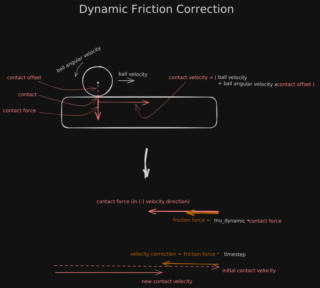
void CollisionConstraint::applyConstraintVelocity(float substepSeconds
    const ObjectBounds& objectA, PhysicsState& physicsA,
    const ObjectBounds& objectB, PhysicsState& physicsB
) {
    // cache position related stuff
    const glm::vec3 positionA { objectA.getPositionWorld() };
    const glm::vec3 positionB { objectB.getPositionWorld() };
    const glm::quat orientationA { objectA.getOrientationWorld() };
    const glm::quat orientationB { objectB.getOrientationWorld() };
    const glm::vec3 contactPositionA { positionA + orientationA * mRelativePointContactA };
    const glm::vec3 contactPositionB { positionB + orientationB * mRelativePointContactB };

    // discover just how fast the contact points on each surface are moving
    // relative to each other
    const glm::vec3 pointVelocityA { physicsA.mVelocity + glm::cross(
        physicsA.mAngularVelocity,
        contactPositionA - positionA
    ) };
    const glm::vec3 pointVelocityB { physicsB.mVelocity + glm::cross(
        physicsB.mAngularVelocity,
        contactPositionB - positionB
    ) };
    const glm::vec3 pointVelocityAB { pointVelocityA - pointVelocityB };
    const float bounceVelocity { glm::dot(pointVelocityAB, mContactNormal) };
    const glm::vec3 tangentialVelocity {
        pointVelocityAB - bounceVelocity * mContactNormal
    };

    // derive the impulse required to fix our velocities
    const float lagrangeCollision { getLagrangeDelta().at(0) };
    const float forceNormal { lagrangeCollision / (substepSeconds * substepSeconds) };
    const glm::vec3 velocityCorrection {
        -glm::normalize(tangentialVelocity) * glm::min(
            glm::abs(substepSeconds * coefficientFrictionDynamic * forceNormal),
            glm::length(tangentialVelocity)
        )
    };
    const glm::vec3 impulseFriction {
        velocityCorrection / (generalizedInverseA + generalizedInverseB)
    };

    // apply the impulse
    physicsA = applyImpulsePhysics(
        objectA,
        physicsA,
        impulseFriction,
        contactPositionA
    );
    physicsB = applyImpulsePhysics(
        objectB,
        physicsB,
        -impulseFriction,
        contactPositionB
    );
}

Note:

My implementation diverges a little from the formulae shown in (33), in the paper, here.

I did need to find the proportion of the impulse that would affect the center of mass, which you see in impulseLinear below, to keep the simulation from misbehaving.

PhysicsState applyImpulsePhysics(
    const ObjectBounds& object,
    PhysicsState physics,
    const glm::vec3& impulsePositional,
    const glm::vec3& impulsePoint
) {
    const glm::vec3 position { object.getPositionWorld() };
    const glm::vec3 impulsePointRelative { impulsePoint - object.getPositionWorld() };
    const glm::vec3 toCenter { glm::normalize(-impulsePointRelative) };
    const glm::vec3 impulseLinear { glm::dot(impulsePositional, toCenter) * toCenter };
    const glm::vec3 deltaVelocity { impulseLinear * physics.mMassInverse };
    physics.mVelocity += deltaVelocity;

    const glm::vec3 impulseRotational { glm::cross(
        impulsePointRelative,
        impulsePositional
    ) };
    physics = applyImpulsePhysics(object, physics, impulseRotational);

    return physics;
}

PhysicsState applyImpulsePhysics(
    const ObjectBounds& object,
    PhysicsState physics,
    const glm::vec3& impulseRotational
) {
    const glm::quat orientation { object.getOrientationWorld() };
    const glm::vec3 impulseLocal { glm::inverse(orientation) * impulseRotational };
    const glm::vec3 deltaVelocityAngular { orientation * (physics.mRotationalInertiaInverse * impulseLocal) };
    physics.mAngularVelocity += deltaVelocityAngular;
    return physics;
}

Note:

While not covered in this post, you can use the same type of velocity constraint to model restitution.

One more physics update update

The velocity correction applies after the velocity derivation step. Our high level physics substep loop must change accordingly:

void PhysicsSystem::onSimulationStep(uint32_t timestepMillis) {
    // other stuff

    // ...

    for(auto substep { 0 }; substep < mSubsteps; ++substep) {
        // prediction step and position constraints

        // ...

        deriveVelocities(substepInterval);

        // !!!!!! -> here's where we'll call our applyConstraintVelocity function
        applyVelocityConstraints(substepInterval);
    }

    // ...

    // more stuff
}

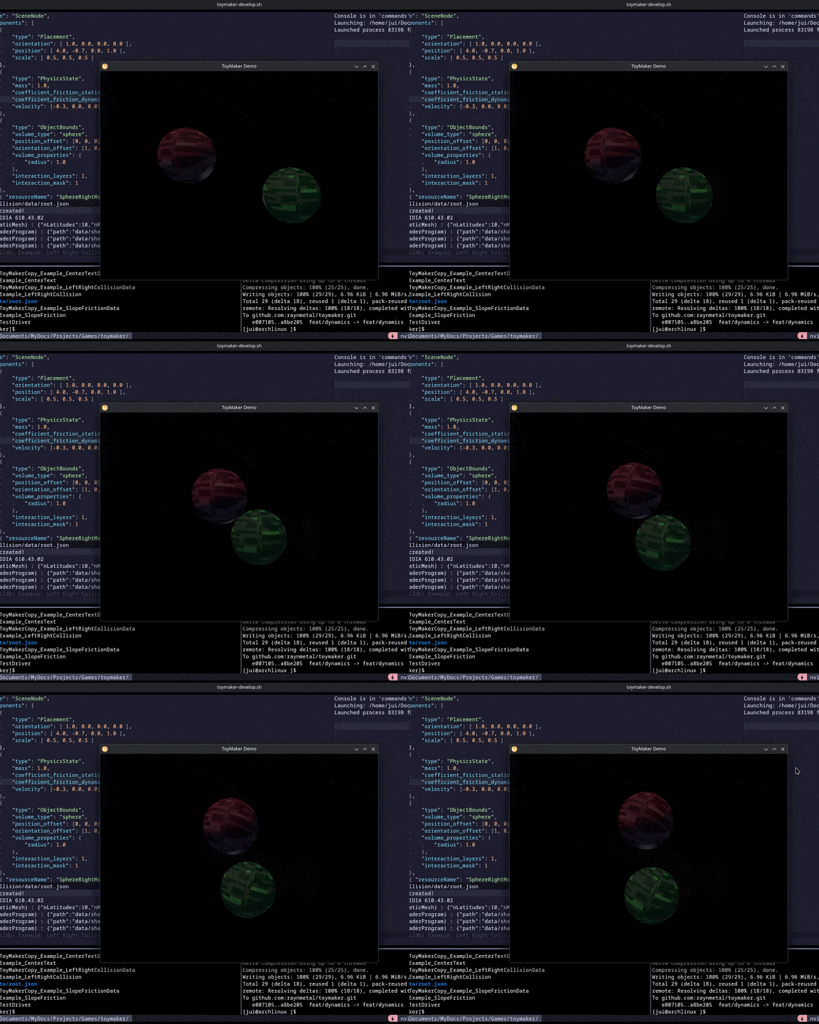
Once we have both static and dynamic friction correctly set up, this is what we finally get:

A note about broad phase collision detection

While GJK and EPA are very good for what they are, they are quite computationally expensive. We’ll want to minimize the number of times we perform these operations as much as possible so that our simulation runs well in real time.

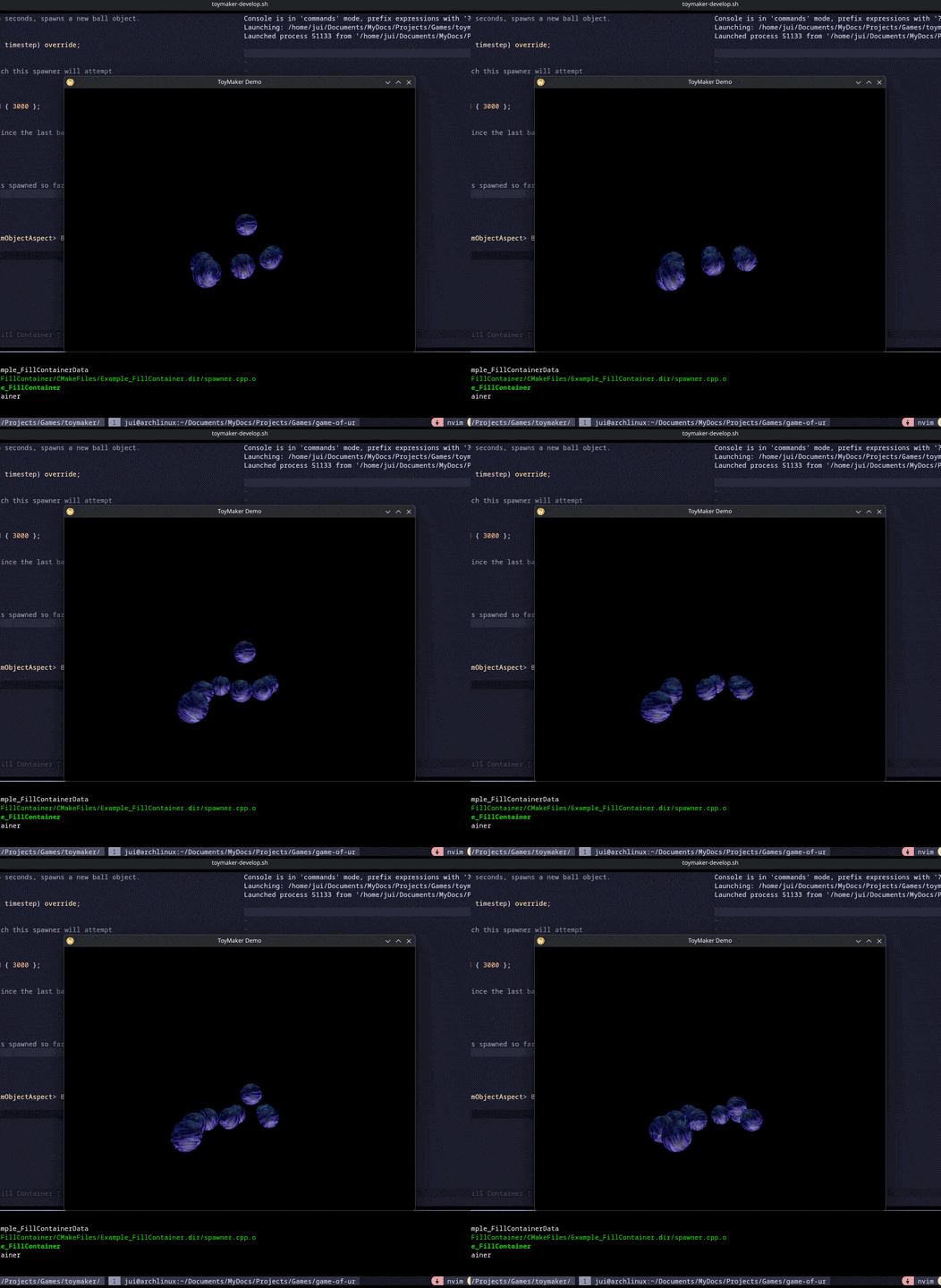
ToyMaker already has a spatial query system that allows us to make fast AABB queries about the scene. It does this by storing object AABBs in a hierarchical data structure called an Octree. There are many other spatial indexing structures one can use instead, however.

We can make a spatial query with each physics object to discover, given the object’s velocity, what other objects it’s likely to collide with within the next physics update. We can then create collision constraints for this frame only for the pairs found through this query. A combination of this technique, as well as a technique called Sweep-and-Prune, applied at each substep, improves the simulation’s performance tremendously.

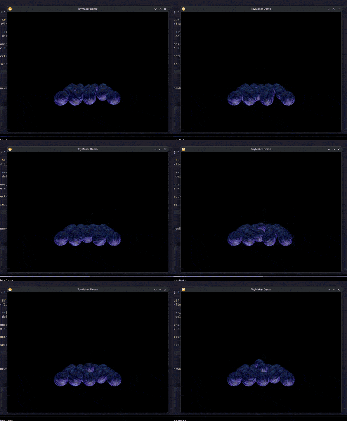
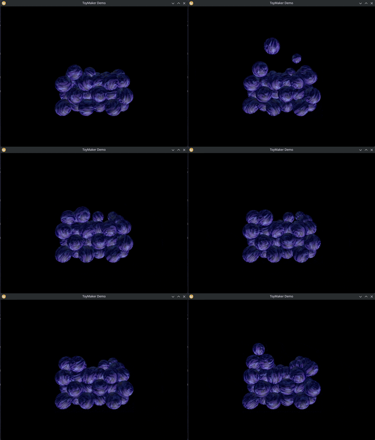
Techniques that perform a computationally cheaper but coarser kind of collision detection to reduce the usage of more accurate but expensive collision tests are collectively called Broad-Phase Collision Detection techniques.

References

• Physics introduction - Godot Engine 4.7 documentation in English – An overview of physics data as represented in Godot, useful for learning how popular engines tackle this task.

• Object/Object Intersections - realtimerendering.com – An extensive collection of links to intersection test techniques for different pairs of shapes.

• Implementing GJK (2006) - Casey Muratori – Video lecture giving a simple breakdown of how GJK works, and how it can be implemented.

• Computing Distance - Erin Catto – Slides that are presumably connected with a talk given at GDC, whose video I could not find. Covers everything from GJK’s rationale to its implementation in easy non-academic language, with plenty of diagrams.

• Game Physics: Contact Generation (EPA) - Allen Chou – Article describing the Expanding Polytope Algorithm, or EPA, for finding collision contact points using the simplex found with GJK.

• Detailed Rigid Body Simulation with Extended Position Based Dynamics - Matthias Müller, Miles Macklin, Nuttapong Chentanez, Stefan Jeschke, Tae-Yong Kim – The paper on the realtime physics simulation approach, XPBD, talked about in this article.

• Ten Minute Physics - Matthias Müller – Index of educational physics programming videos, many of them closely connected with the XPBD paper.

• Impulse-Based Dynamic Simulation - Brian Mirtich – A paper on impulse-based physics solvers as seen in most current physics engines. The appendix contains a very useful collection of derivations for various 3D physics formulae.

• Introduction to Octrees - Eric Nevala – An introduction to spatial partitioning algorithms in general, with a guide to building octrees in particular.

• Advanced Octrees 3: non-static Octrees - David Geier – A very short article which talks about how to dynamically update the region encompassed by an octree in response to changes in a scene.

• Sort, sweep, and prune: Collision detection - leanrada – An explanation of Sweep-and-Prune, a popular broad-phase collision detection algorithm.